Introduction
This tutorial is based on multiple chapters of “Text Mining with R: A Tidy Approach” by Julia Silge and David Robinson.
Throughout this tutorial, we will use the tidytext package to analyze
text data, in particular the contents of Alice in Wonderland and
Winnie-the-Pooh. This book and many others are available via the
gutenberg_download() function in the gutenbergr package, which
provides access to the Project Gutenberg collection of public domain
books.
# install.packages("tidytext")
# install.packages("gutenbergr")
library(tidyverse)
library(tidytext)
library(gutenbergr)

# Download books based on their Gutenberg ID
# https://gutenberg.org/ebooks/19033
# https://gutenberg.org/ebooks/67098
books <- gutenberg_download(c(19033, 67098), mirror = "http://mirror.csclub.uwaterloo.ca/gutenberg/")
Representing text as data
Tidy text format
Currently in the books tibble, each row represents a line of text from
one of the books. It is often useful to represent text data in a tidy
format, where each row represents a word or token, as then we can apply
data wrangling operations on the word level. We can use the
unnest_tokens() function from the tidytext package to easily split
the text into words, or into other levels of analysis such as
characters, sentences or paragraphs. This function also takes care of
removing punctuation, converting words to lowercase, and dropping empty
rows. Before tokenizing, we may want to remove the contents of the
titlepage, as the actual book contents only start on line 38 for Alice
in Wonderland and line 79 for Winnie-the-Pooh.
# remove title page and add book title variable
books_content <- books |>
  # add book title
  mutate(book_title = ifelse(gutenberg_id == 19033, "Alice", "Winnie")) |>
  # restart counting row numbers for each book
  group_by(book_title) |>
  filter((book_title == "Alice" & row_number() >= 38) |
           (book_title == "Winnie" & row_number() >= 79)) |>
  ungroup()

words <- books_content |>
  # split books into words
  unnest_tokens(output = word, input = text)
You may notice that not all words are completely clean or relevant: some are surrounded by underscores and some are numbers. We can clean these up manually with regular expressions.
words <- words |>
  mutate(word = str_remove_all(word, "_")) |>
  filter(!str_detect(word, "^\\d+$"))
Term frequency
The term frequency (tf) of a word is the number of times it appears in a document, divided by the total number of words in the document. It is simply the result of counting the number of times a word appears in the document.
tf <- words |>
  # count the number of times each word appears in each book
  count(book_title, word) |>
  # divide by number of words in each book
  group_by(book_title) |>
  mutate(tf = n / sum(n)) |>
  ungroup()
Term frequency - inverse document frequency (tf-idf)
The inverse document frequency (idf) of a word is the logarithm of the
total number of documents divided by the number of documents that
contain the word. It is a measure of how unique or rare a word is across
the entire corpus. The intuition for why idf matters is that words that
appear in many documents are less informative than words that appear in
only a few documents. Therefore we often combine tf and idf into a
single metric called term frequency-inverse document frequency (tf-idf),
which is the product of tf and idf. The bind_tf_idf() function from
the tidytext package can be used to calculate tf-idf values (the
function also generates tf and idf separately).
tf_idf <- words |>
  count(book_title, word) |>
  bind_tf_idf(word, book_title, n)
Document-term matrix
Documents (in out case, books) can be represented as a document-term
matrix, where each row represents a document and each column represents
a word. The value in each cell is equal to the frequency of the word in
the document. This matrix is sometimes called the bag-of-words
representation of the text data (although sometimes that contains 0/1
values based on whether the word appears in the document), because it
ignores the ordering of the words in the text. These matrices can be
created using the cast_dtm() function from the tidytext package.
Note that these matrices can get very large depending on the size of the
vocabulary and the number of documents. Our data has less than 3000
unique words and 2 documents, so it is manageable.
# DTM with pivot_wider() (generic tibble)
dtm <- words |>
  count(book_title, word) |>
  pivot_wider(names_from = word, values_from = n, values_fill = 0)

# DTM with cast_dtm() (DocumentTermMatrix object)
dtm <- words |>
  count(book_title, word) |>
  cast_dtm(document = book_title, term = word, value = n)
Text analysis
Visualize word frequencies
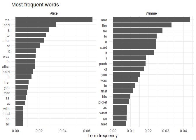
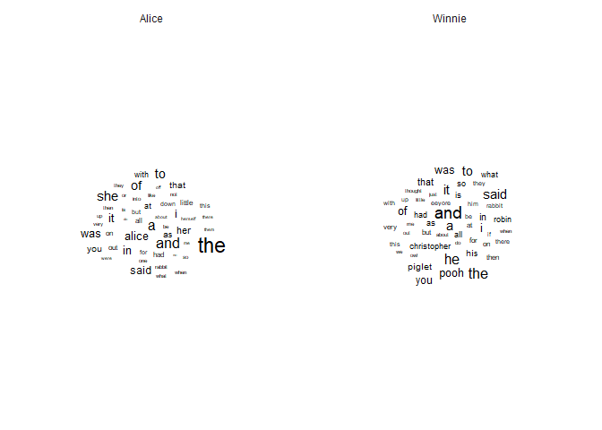
The easiest way to represent the contents of a document is to show the
most frequent words. We can use a bar chart to show the words with
highest term frequency in each book, or use a word cloud where the size
of the word is proportional to its frequency (using the ggwordcloud
package).
library(ggwordcloud)

# Most frequent words
tf_idf |>
  group_by(book_title) |>
  slice_max(tf, n = 20) |>
  ggplot(aes(tf, reorder_within(word, tf, book_title))) +
  geom_col() +
  facet_wrap(~book_title, scales = "free") +
  scale_y_reordered() +
  labs(x = "Term frequency", y = NULL, title = "Most frequent words") +
  theme_minimal()
# Word cloud
tf |>
  group_by(book_title) |>
  top_n(50, tf) |>
  ggplot(aes(label = word, size = tf)) +
  geom_text_wordcloud() +
  facet_wrap(~book_title) +
  theme_minimal()
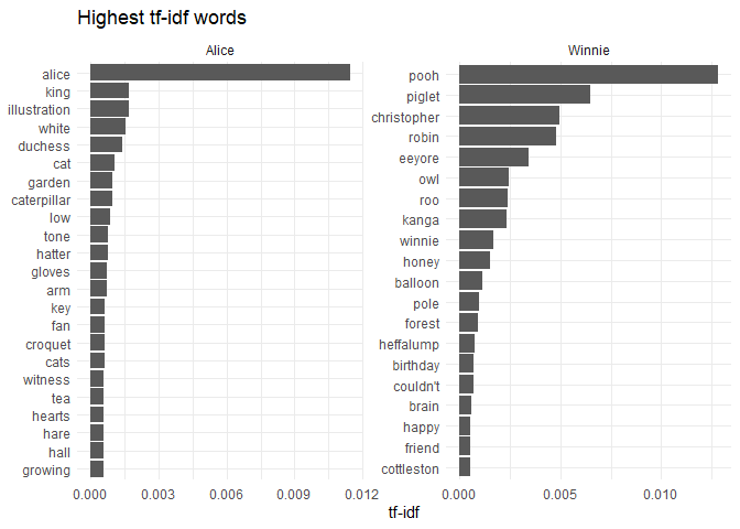
Using simple word frequencies is often uninformative because common words like “the” or “and” will dominate the results. One way to address this problem is to display the words with highest tf-idf values: in the case of two books, this will show the words that are unique to each book, as words that show up in all document have idf=tf-idf=0.
tf_idf |>
  group_by(book_title) |>
  slice_max(tf_idf, n = 20) |>
  ggplot(aes(tf_idf, reorder_within(word, tf_idf, book_title))) +
  geom_col() +
  facet_wrap(~book_title, scales = "free") +
  scale_y_reordered() +
  labs(x = "tf-idf", y = NULL, title = "Highest tf-idf words") +
  theme_minimal()
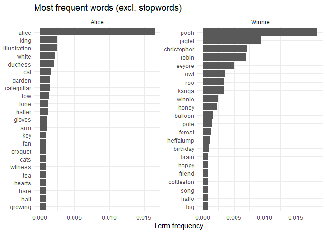
An alternative method is to remove common words (called stopwords) from
the analysis, using a stopword list. tidytext provides a list of
stopwords with the get_stopwords() function, which can be used to
filter out common words from the analysis.
stopwords <- get_stopwords() |> pull(word)

tf_idf |>
  group_by(book_title) |>
  # remove stopwords
  filter(!word %in% stopwords) |>
  slice_max(tf_idf, n = 20) |>
  ggplot(aes(tf, reorder_within(word, tf, book_title))) +
  geom_col() +
  facet_wrap(~book_title, scales = "free") +
  scale_y_reordered() +
  labs(x = "Term frequency", y = NULL, title = "Most frequent words (excl. stopwords)") +
  theme_minimal()
Bigrams, n-grams
Bigrams are pairs of words that appear next to each other in a document;
n-grams are sequences of n words. They can be useful to capture the
context in which words appear, as the meaning of a word can depend on
the words that surround it. By specifying the token argument in the
unnest_tokens() function, we can split the text into bigrams or
n-grams.
bigrams <- books_content |>
  unnest_tokens(bigram, text, token = "ngrams", n = 2)
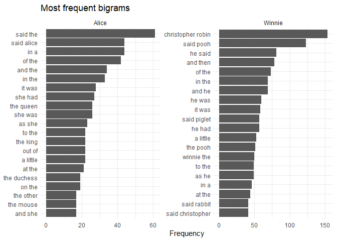
We can visualize the most common bigrams the same way we did for unigrams (single words).
bigrams |>
  drop_na() |>
  count(book_title, bigram) |>
  group_by(book_title) |>
  slice_max(n, n = 20) |>
  ggplot(aes(n, reorder_within(bigram, n, book_title))) +
  geom_col() +
  facet_wrap(~book_title, scales = "free") +
  scale_y_reordered() +
  labs(x = "Frequency", y = NULL, title = "Most frequent bigrams") +
  theme_minimal()
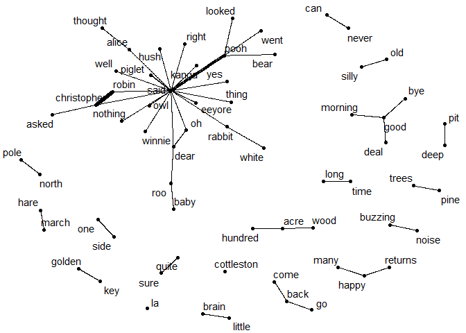
In addition, we can make use of the extra context information provided
by bigrams, and visualize which words are most likely to appear after a
given word. For that, we need to separate the bigrams into two columns,
one for the first word and one for the second word. To keep the
vocabulary relatively small, we will only consider bigrams where neither
of the words is a stopword. We can use these frequencies to create a
network visualization of the most common bigrams with the igraph and
ggraph packages.
library(igraph)
library(ggraph)

# create graph object
bigram_graph <- bigrams |>
  drop_na() |>
  # separate bigrams into two columns
  separate(bigram, c("word1", "word2"), sep = " ") |>
  # remove stopwords
  filter(!word1 %in% stopwords & !word2 %in% stopwords) |>
  # count word frequencies
  count(word1, word2) |>
  # remove bigrams that appear less than 5 times
  filter(n > 5) |>
  # create graph object
  graph_from_data_frame()

# plot graph
ggraph(bigram_graph, layout = "fr") +
  geom_edge_link(aes(edge_width = n), show.legend = FALSE) +
  geom_node_point() +
  geom_node_text(aes(label = name), repel = TRUE) +
  scale_edge_width(range = c(0.1, 2)) +
  theme_void()
Sentiment analysis
Sentiment analysis is the process of determining the sentiment of a
piece of text, i.e. whether it is positive, negative, or neutral. One
way to do this is to use a sentiment lexicon, which is a list of words
and their associated sentiment scores. There are multiple different
sentiment lexicons available, such as Bing, AFINN, and NRC. These differ
in their training data and the sentiment categories they use, but are
all available with the get_sentiments() function. So we can use the
tidy words tibble and merge it with the sentiment lexicon to assign
sentiment scores to each word.
# get sentiment lexicons
bing <- get_sentiments("bing")
afinn <- get_sentiments("afinn")

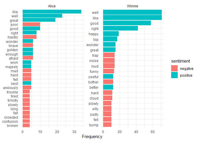
# plot the most common positive and negative words with the Bing lexicon
words |>
  inner_join(bing, by = "word") |>
  count(book_title, word, sentiment) |>
  group_by(book_title, sentiment) |>
  slice_max(n, n = 10) |>
  ggplot(aes(n, reorder_within(word, n, book_title), fill = sentiment)) +
  geom_col() +
  scale_y_reordered() +
  labs(x = "Frequency", y = NULL) +
  facet_wrap(~book_title, scales = "free") +
  theme_minimal()
# calculate sentiment scores per book with the AFINN lexicon
words |>
  count(book_title, word) |>
  inner_join(afinn, by = "word") |>
  # calculate each word's contribution to the sentiment score
  mutate(value_n = value * n) |>
  group_by(book_title) |>
  # calculate the sentiment score for each book (sum of sentiment scores / number of words)
  summarize(score = sum(value_n) / sum(n))
## # A tibble: 2 × 2
##   book_title score
##   <chr>      <dbl>
## 1 Alice      0.124
## 2 Winnie     0.810
Topic modelling
Topic modelling is a method to discover the topics that are present in a
collection of documents. It is an unsupervised learning method, meaning
that it does not require labeled data. One popular topic modelling
method is latent Dirichlet allocation (LDA), which assumes that each
document is a mixture of different topics, and each topic is a mixture
of words. The LDA() function from the topicmodels package can be
used to fit an LDA model to a document-term matrix. The function
requires a document-term matrix as created by cast_dtm(), so first we
should create a clean version of our previous dtm object (remove
stopwords).
Before we fit a model, we need to decide how many topics to use. If we have previous expectations about what results we want to see, we can choose a specific number of topics, otherwise we can try multiple values until we find sensible results. The model also includes a random initialization step, so it is a good idea to set a seed to ensure that we get the same results every time. In this case, we might try to fit a model with 2 topics if we hope that the model can separate the topics of the two documents.
library(topicmodels)

dtm <- words |>
  count(book_title, word) |>
  filter(!word %in% stopwords) |>
  cast_dtm(document = book_title, term = word, value = n)

# fit LDA model with 2 topics
lda <- LDA(dtm, k = 2, control = list(seed = 1))
When interpreting LDA results, we consider two sets of parameters: the
document-topic matrix and the topic-word matrix. The document-topic
matrix tells us how much of each topic is present in each document,
while the topic-word matrix tells us which words are associated with
each topic. We can use the tidy() function from the topicmodels
package to extract these matrices into a tidy format, specifying
matrix = "beta" for the topic-word matrix and matrix = "gamma" for
the document-topic matrix.
topic_word <- tidy(lda, matrix = "beta")
document_topic <- tidy(lda, matrix = "gamma")
The topic-word matrix helps us give meaning to the topics by showing which words are the most strongly associated with each topic. We can plot these word probabilities to visualize the topics.
topic_word |>
  group_by(topic) |>
  slice_max(beta, n = 10) |>
  ggplot(aes(beta, reorder_within(term, beta, topic))) +
  geom_col() +
  facet_wrap(~topic, scales = "free") +
  scale_y_reordered() +
  labs(x = "Per-topic-per-word probability", y = NULL) +
  theme_minimal()
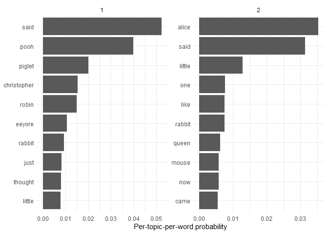
It seems like the topics can separate the two books well, although it might not succeed with a different random seed.
The per-document-per-topic probabilities confirm that the the documents are clearly split into topics, with each having a near-1 probability for one topic and near-0 for the other.
document_topic |>
  pivot_wider(names_from = topic, values_from = gamma)
## # A tibble: 2 × 3
##   document        `1`        `2`
##   <chr>         <dbl>      <dbl>
## 1 Alice    0.00000788 1.00
## 2 Winnie   1.00       0.00000338
Nevertheless, topic modelling can be very useful for larger collections of documents, where it can help to identify the main themes present in the corpus.